Core Analysis Tools
The platform provides form-driven analysis pipelines for single-dataset statistics and machine learning, multi-omics integration, and pathway enrichment.
Single-Omics Analysis
The Analysis Configuration page runs correlation analysis, ordination, clustering, statistical tests, and machine-learning methods such as Random Forests against a selected dataset.
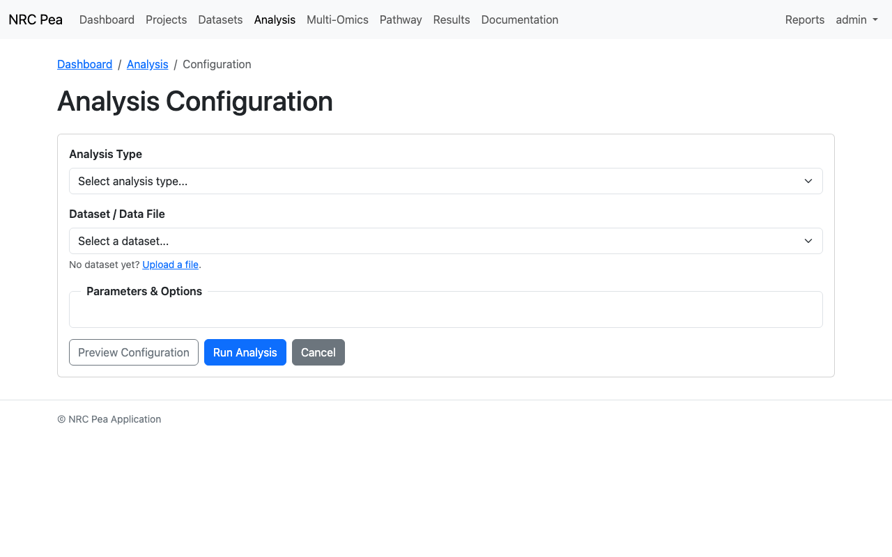
Analysis Configuration Interface
Multi-Omics Integration
Multi-Omics configurations enable users to fuse orthogonal datasets (e.g. transcriptomics with metabolomics) to discover shared latent factors with MOFA2 or to discriminate pre-defined sample classes across blocks with DIABLO. MOFA2 is a pure-Python unsupervised method; DIABLO is a supervised sparse method that requires R and the mixOmics package. See the Multifactor Analysis Guide for method choice, parameters and interpretation.
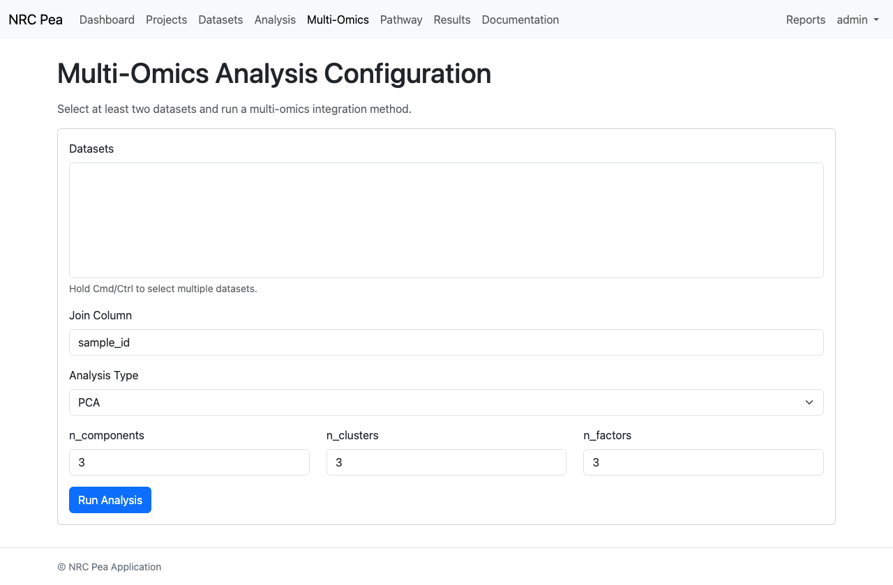
Multi-Omics Setup
Pathway Analysis
The Pathway Analysis tool maps a gene list onto biological databases (GO, KEGG, Reactome) with Over-Representation Analysis (ORA), or scores a ranked list against gene sets with GSEA.
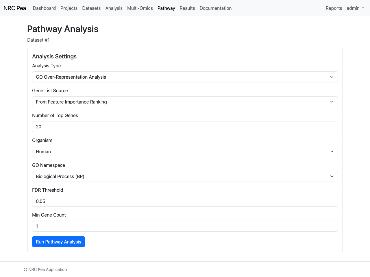
Pathway Investigation Panel
Method Catalogue
Every analysis method offered by the live server is listed below, grouped by category. Each entry names the data the method needs. The same registry drives the method selection page, so this list always matches what the server can actually run.
Data Preparation
| Method | What it does | Required input |
|---|---|---|
| Preprocessing | Impute missing values, normalise features and handle outliers. Produces a derived dataset for downstream use.
POST fields:
dataset_id,
min_col_fraction,
missing_strategy,
normalization,
outlier_handling,
outlier_method,
target_col
|
One dataset with numeric columns. |
| Feature Selection | Rank and select the most informative features (importance, SelectKBest, RFE, SFS and more). Produces a derived dataset with the selected features plus the target.
POST fields:
dataset_id,
feature_selection_method,
fs_estimator,
fs_threshold,
k,
target_col
|
One dataset with a numeric target column. |
| Feature Engineering | Create derived features — ratios, sums, products, means, log1p, polynomial interactions, longitudinal summaries, one-hot columns, or a wide→long reshape — saved as a new dataset for downstream analysis.
POST fields:
dataset_id,
fe_columns,
fe_degree,
fe_id_cols,
fe_interaction_only,
fe_name,
fe_operation,
fe_prefix
|
Numeric columns (plus a group column for one-hot). |
Statistical Analysis
| Method | What it does | Required input |
|---|---|---|
| Correlation Analysis | Compute a pairwise correlation matrix (Pearson, Spearman or Kendall) across all numeric features.
POST fields:
dataset_id,
correlation_method
|
One dataset with at least two numeric columns. |
| Univariate Screening | Pre-modeling screening: per-feature Pearson, Spearman and ANOVA F statistics against a target with FDR correction. Produces a derived dataset of significant features.
POST fields:
dataset_id,
fdr_threshold,
target_col
|
One dataset with a numeric target column. |
| t-Test | Compare the mean of a numeric variable between two groups (independent or paired samples).
POST fields:
dataset_id,
alpha,
group_col,
paired,
value_col
|
A numeric value column and a group column with exactly 2 groups. |
| One-way ANOVA | Compare the mean of a numeric variable across two or more groups.
POST fields:
dataset_id,
alpha,
group_col,
value_col
|
A numeric value column and a group column with 2+ groups. |
| Chi-Square Test | Test whether two categorical variables are independent using a contingency table of observed counts.
POST fields:
dataset_id,
alpha,
column_a,
column_b
|
Two categorical columns. |
| Mann-Whitney U Test | Non-parametric comparison of a numeric variable between two groups (no normality assumption).
POST fields:
dataset_id,
alpha,
group_col,
value_col
|
A numeric value column and a group column with exactly 2 groups. |
| Kruskal-Wallis Test | Non-parametric comparison of a numeric variable across two or more groups.
POST fields:
dataset_id,
alpha,
group_col,
value_col
|
A numeric value column and a group column with 2+ groups. |
| Repeated-Measures ANOVA | Within-subject ANOVA over wide-format timepoint columns (e.g. JUN/JUL/AUG cover), with an optional between-subject factor. Saves the melted long table as a derived dataset.
POST fields:
dataset_id,
between_col,
timepoint_cols
|
Two or more numeric timepoint columns, one row per subject. |
| Count GLM (Poisson / NB) | Generalised linear model for count responses — Poisson or negative-binomial family with categorical predictors automatically dummy-coded.
POST fields:
dataset_id,
glm_family,
nb_alpha,
predictor_cols,
value_col
|
A non-negative count column and one or more predictors. |
| Mixed-Effects Model (LMM) | Linear mixed model with a random intercept per group — handles nested/repeated designs such as plots within pastures or ranches.
POST fields:
dataset_id,
fixed_col,
group_col,
value_col
|
A numeric response, a fixed effect, and a grouping column. |
| Clustering | Group plots or samples into clusters (K-Means or hierarchical) on z-scored numeric features. Saves a derived dataset with a cluster column for downstream use (e.g. management zones).
POST fields:
dataset_id,
cluster_method,
feature_cols,
linkage,
n_clusters
|
One dataset with at least one numeric column. |
| Ordination (PCA / PCoA / NMDS) | Reduce a samples-by-features table to a 2-D ordination: PCA, principal coordinates analysis (PCoA) or non-metric multidimensional scaling (NMDS) with a choice of distance metric.
POST fields:
dataset_id,
color_col,
distance_metric,
feature_cols,
n_components,
ordination_method
|
One dataset with at least two numeric columns. |
Community Ecology
| Method | What it does | Required input |
|---|---|---|
| Alpha Diversity | Per-sample diversity indices (richness, Shannon, Simpson, Pielou evenness) over a community matrix; optional group summaries. Saves indices as a derived dataset.
POST fields:
dataset_id,
feature_cols,
group_col
|
A samples-by-features community matrix. |
| Beta Diversity (PERMANOVA + ANOSIM) | Pairwise distance matrix (Bray-Curtis, Jaccard, ...) with PERMANOVA and ANOSIM group-composition tests plus a distance heatmap.
POST fields:
dataset_id,
distance_metric,
feature_cols,
group_col,
n_perm
|
Community matrix plus a categorical group column. |
| Mantel Test | Correlates two distance matrices (e.g. community dissimilarity vs environmental distance) with a permutation p-value.
POST fields:
dataset_id,
distance_metric,
env_cols,
env_metric,
feature_cols,
n_perm
|
Two non-overlapping sets of numeric columns. |
| Indicator Species (IndVal) | Dufrene-Legendre indicator values: which features are specific to and frequent within each group.
POST fields:
dataset_id,
feature_cols,
group_col,
n_perm
|
Community matrix plus a categorical group column. |
| Morans I (Spatial Autocorrelation) | Tests whether a variable is spatially clustered using k-nearest-neighbour weights and a permutation p-value.
POST fields:
dataset_id,
k,
lat_col,
long_col,
n_perm,
value_col
|
Latitude, longitude and a numeric value column. |
Machine Learning
| Method | What it does | Required input |
|---|---|---|
| Random Forest | Multi-split Random Forest regression with feature importance, optional univariate screening, permutation tests and SHAP values.
POST fields:
dataset_id,
categorical_encoding,
fdr_threshold,
n_estimators,
n_splits,
permutation_repeats,
random_state,
run_permutation,
run_shap,
run_univariate,
target_col,
test_size
|
One dataset with a numeric target column. |
| Model Comparison | Benchmark multiple regressors (linear, trees, boosting, SVR, neural net) under the same cross-validation splits.
POST fields:
dataset_id,
categorical_encoding,
model_keys,
n_splits,
target_col,
test_size
|
One dataset with a numeric target column. |
| Full Pipeline | End-to-end run: preprocessing, feature engineering and selection, model training, evaluation and interpretation.
POST fields:
dataset_id,
categorical_encoding,
fdr_threshold,
feature_selection_method,
k,
missing_strategy,
n_estimators,
n_splits,
normalization,
outlier_handling,
outlier_method,
permutation_repeats,
run_permutation,
run_shap,
target_col,
test_size
|
One dataset with a numeric target column. |
Multi-Omics Integration
| Method | What it does | Required input |
|---|---|---|
| PCA (Multi-Omics) | Per-block principal component analysis with an integrated overview. | Multiple omics blocks (wide table or separate files). |
| SNF optional dep: snfpy | Similarity Network Fusion — integrates blocks into one sample-similarity network. | Multiple omics blocks. Requires the snfpy package. |
| MOFA+ optional dep: mofapy2 | Multi-Omics Factor Analysis — latent factors driving variation across views. | Multiple omics blocks. Requires the mofapy2 package. |
| MOFA2 optional dep: mofapy2 | Unsupervised factor discovery across multiple omics views (full pipeline). | Multiple omics blocks. Requires the mofapy2 package. |
| DIABLO optional dep: rscript | Supervised multi-block discrimination of outcome classes (mixOmics). | Multiple omics blocks and a categorical outcome. Requires R + mixOmics. |
| CCA | Canonical Correlation Analysis — maximally correlated components across blocks. | Two or more omics blocks. |
| NMF | Non-negative Matrix Factorisation — parts-based decomposition per block. | Omics blocks with non-negative values. |
Genomics & Pathway
Minimum data sizes: most statistical tests need at least 3 observations per group; ordination needs at least 3 complete rows; repeated-measures needs 2+ timepoint columns; MOFA2/DIABLO need 2+ blocks with 6+ shared samples each; chi-square needs a 2×2 (or larger) joint contingency table with expected counts preferably above 5.
Parameter Reference Guide
Detailed technical specifications for the core configuration parameters available in the analysis modules.
Analysis Type
Defines the high-level methodology (e.g., Random Forest, Correlation, or GWAS Screening). Controls which downstream parameters are visible.
Number of Estimators
The number of decision trees in the ensemble model. Higher values lead to more stable models but require more memory.
Number of CV Splits
The $k$ partitions used for $k$-fold cross-validation. Typical academic baseline is 5 or 10.
Test Size
Proportion of the dataset used for validation (e.g., 0.2 represents 20% for testing).
Random State (Seed)
Integer seed value ensuring that stochastic operations (like dataset splitting) are identically reproducible across runs.
Categorical Feature Encoding
How non-numeric feature columns are converted before modeling: Exclude drops them, Integer maps each level to a number (1, 2, 3…), and One-hot expands each level into its own 0/1 column (e.g., RANCH_KINSELLA).
Correlation Method
Determines how to measure feature association: Pearson (linear), Spearman (rank), or Kendall (robust).
FDR Threshold (q-value)
The false discovery rate cutoff (Benjamini-Hochberg) for reporting significant biological findings.
Permutation Repeats
The number of shuffles performed to generate internal null distributions for feature importance significance testing.
SHAP Analysis Coverage
Enables calculation of Shapley values for model local interpretability, identifying variable contribution per sample.
Gene List Source
Input selection for enrichment. Utilizes high-ranking features from Random Forest or manually curated user lists.
Feature Subset Size (Top N)
The count of highest-ranking genes to include in ORA calculations.
Minimum Column Fraction
Fraction of numeric columns a row must be outlying in before IQR/Z-Score detection flags it. Higher values are more conservative on wide datasets.
Manual Gene List
Gene or feature identifiers typed or pasted directly — one symbol per line or comma-separated. Used when Gene List Source is "Manual Gene Input".
Biological Organism
Species context for gene ID mapping (e.g., Human vs specialized genomic backends).
GO Namespace
Specifies which Gene Ontology branch to query: Biological Process, Molecular Function, or Cellular Component.
Minimum Overlap Threshold
The minimum number of provided genes required within a pathway to trigger statistical testing.
Data & Target Selection
Dataset Selection
The primary data source for the analysis. All preprocessing, statistics, and modeling are executed against the records in this file. Datasets are uploaded via the Datasets page and can be filtered by project.
Target Column (Dependent Variable)
The outcome variable (Y) to predict or correlate against. For regression models this must be a continuous numeric column; leave blank to auto-detect the first numeric column.
Single-Omics Toggles
Normalize Data
Scales feature values before analysis so that variables measured on large ranges do not dominate distance- or variance-based models. Recommended when columns mix different units or magnitudes.
Pearson Correlation
Univariate screen measuring the linear association between each feature and the target. Fast and interpretable; assumes roughly normal distributions.
Spearman Correlation
Rank-based univariate screen for monotonic (not necessarily linear) relationships. More robust to outliers and skewed data than Pearson.
ANOVA F-test
Compares feature means across groups defined by a categorical target to flag variables that differ significantly between classes or conditions.
Pipeline Editor — Preprocessing
Missing Values
How empty cells are handled before modeling: keep them, or impute each column with its mean (default), median (robust to outliers), or mode (for categorical data).
Normalization
Rescales feature magnitudes: min-max maps each column to the 0–1 range; z-score standardises to zero mean and unit variance.
Outlier Detection
The algorithm used to flag anomalous samples: IQR (simple rule), IsolationForest, LOF, EllipticEnvelope, OneClassSVM, or DBSCAN.
Outlier Handling
What to do with detected outliers: remove the rows, keep them, winsorize extreme values to percentile bounds, or impute with the column median/mean.
Outlier Timing
When outlier handling is applied relative to the train/test split. Training only avoids leaking information from test samples into the decision.
Pipeline Editor — Feature Engineering
Log Transform
Applies log(x) to numeric features, compressing right-skewed distributions common in count and concentration data.
Sqrt Transform
Applies the square-root transform — a milder variance-stabilising correction than log, suited to moderately skewed count data.
Reciprocal Transform
Applies 1/x, strongly shrinking large values and spreading small ones. Useful for extremely right-skewed positive data.
Power Transform (Yeo-Johnson)
Estimates an optimal power transform per feature to approximate a normal distribution; unlike Box-Cox it supports zero and negative values.
Quantile Transform
Maps each feature to a uniform or normal distribution via its empirical quantiles. Robust to any input distribution but destroys relative distances between values.
Polynomial Features
Generates interaction and power terms between features up to the chosen degree, letting the model capture non-linear relationships (e.g., x1·x2, x12).
Polynomial Degree
The maximum power of generated polynomial terms. Higher degrees grow the feature count rapidly and risk overfitting.
Spline Transform
Expands features into piecewise polynomial basis functions so linear models can fit smooth non-linear trends such as dose-response curves.
KBins Discretize
Buckets continuous features into discrete intervals, converting numeric variables into categorical bins.
Pairwise Ratios
Creates ratio features between column pairs, exposing proportional or stoichiometric relationships that absolute values hide.
Pipeline Editor — Feature Selection & Model
Feature Selection Method
Strategy for reducing the feature set before modeling: variance threshold, correlation filter, recursive feature elimination (RFE), K-Best scoring, percentile, FDR, or model-based selection.
K Features
The number of top-ranked features retained by the selection method.
Scoring Function
The metric used to rank features during selection: R², F-regression, or mutual information.
Task Type
Regression predicts a continuous numeric outcome; classification predicts discrete categories. The choice determines which model list and metrics apply.
Model
The machine learning algorithm to train. Random Forest is a robust default for tabular omics data; linear models suit well-understood linear relationships. Optional models (XGBoost, LightGBM, CatBoost) appear only when installed.
Hyperparameter Tuning
Searches a parameter grid to find better model settings. Slower than a single fit but often improves predictive performance.
Search Strategy
Grid search evaluates every parameter combination; random search samples combinations and is faster on large grids.
Tuning CV Folds
Number of cross-validation folds used inside the hyperparameter search loop. More folds give stabler estimates at higher compute cost.
Pipeline Editor — Advanced Options
Pre-Modeling Statistics
Runs Pearson, Spearman, and ANOVA screens before modeling to summarise each feature's relationship with the target.
Impurity Importance
Mean decrease in impurity computed inside tree-based models. Fast and built-in, but biased toward features with many distinct values.
Permutation Importance
Shuffles each feature and measures the resulting accuracy drop, giving a model-agnostic estimate of feature contribution.
Categorical Encoding
How non-numeric columns are converted before saving or modeling: keep as-is, map to integer codes, or expand into one-hot dummy columns.
GWAS Pipeline
Encoding Model
How genotypes are converted to numeric values: additive counts effect alleles (0/1/2); dominant and recessive collapse genotypes by inheritance model.
Min MAF
Minimum Minor Allele Frequency. SNPs rarer than this threshold are filtered out as statistically uninformative (default 0.05).
Max SNP Missingness
Maximum fraction of missing genotype calls allowed per SNP before it is dropped from the analysis.
Max Sample Missingness
Maximum fraction of missing genotypes allowed per sample before the sample is excluded.
HWE Threshold
Hardy-Weinberg Equilibrium p-value cutoff. SNPs below it deviate from expected genotype frequencies and may indicate genotyping error.
LD Pruning
Removes highly correlated SNPs in linkage disequilibrium to reduce redundancy and multicollinearity before association testing.
LD r² Threshold
Pairwise correlation cutoff used during LD pruning. SNP pairs above this r² are reduced to a single representative.
Association Method
The regression framework for SNP-trait testing: linear regression for quantitative traits, logistic regression for binary case/control outcomes.
Genomic Control
Applies an inflation-factor correction to p-values to account for population stratification and reduce spurious associations.
Multiple Testing Correction
Controls false positives across many SNP tests. Bonferroni is strict; Benjamini-Hochberg FDR balances discovery rate and error control.
Significance Threshold
The genome-wide p-value cutoff for calling a SNP-trait association significant after multiple-testing correction (conventional: 5×10⁻⁸).
Multi-Omics Integration
Join Column (Primary Key)
The shared variable used to align samples across different omics datasets. It must exist in all selected datasets with matching entry IDs.
Data Layout
How the omics blocks are organised: a single wide table splits columns by prefix; multiple files uses one file per block; transposed has samples in columns and features in rows.
Sample ID Column
The column identifying samples across blocks, used to align rows when joining multiple omics layers.
Block Rule
How columns are assigned to blocks in a single wide table: prefix splits on the first underscore (e.g. ENV_temp → ENV block); manual lets you assign columns explicitly.
Feature ID Column
In transposed layout, the column identifying features (rows). Never auto-detected — it must be specified explicitly.
Outcome Column
The categorical variable DIABLO discriminates. Required for DIABLO; classes with fewer than ~10 members trigger a warning.
Principal Components
Number of latent dimensions extracted during dimensionality reduction (PCA, CCA). More components capture more variance but may include noise.
Cluster Count
The expected number of biological or technical subgroups in the integrated data (e.g., for SNF or K-Means).
Latent Factors
For factor analytic models like MOFA2: the underlying biological drivers or technical variance components spanning multiple omics views.
DIABLO Components (ncomp)
Number of latent components for the multi-block PLS-DA model. More components capture more discriminative structure but risk overfitting.
DIABLO keepX
Number of features retained per block per component in the sparse PLS model. Use the same value for all blocks or specify per-block values.
DIABLO Design Matrix
Controls how blocks are linked: full links all blocks to each other; null treats blocks independently; custom allows pairwise weights.
DIABLO perf Folds
Number of cross-validation folds for the perf() error-rate estimation.
DIABLO perf Repeats
Number of times cross-validation is repeated for balanced error-rate (BER) stability.
DIABLO Random Seed
Integer seed for reproducible DIABLO results.
DIABLO Tuning
Opt-in tuning of keepX via tune.block.splsda. The estimated cost derives from grid_size × ncomp × nrepeat × folds.
MOFA2 Convergence Mode
Controls convergence criteria for the variational EM algorithm: fast stops early; slow runs more iterations for tighter convergence.
MOFA2 dropR2 Threshold
Minimum R-squared contribution for a factor to be retained. Factors explaining less variance than this threshold are pruned.
MOFA2 scale_views
Whether to scale each view to unit variance before fitting. Useful when views have very different magnitudes.
MOFA2 Random Seed
Integer seed for reproducible MOFA2 factor estimation.
Model Predictions
Trained Model File
A pickled scikit-learn compatible model (.pkl, .pickle, .joblib) exported from a previous result. Works for both classification and regression. Only upload models you trust.
Identifier Column
Optional column used to label each row in the prediction output so results can be traced back to individual samples.
Method Pages — Statistical Tests & Selection
Univariate Screening
Runs Pearson, Spearman and ANOVA F tests of every feature against the target with FDR correction. Standalone screening produces a derived dataset containing only the significant features plus the target, ready for downstream preprocessing or modeling.
Value Column
Numeric column whose distribution is compared across groups by t-test, ANOVA, Mann-Whitney or Kruskal-Wallis.
Group Column
Categorical column defining comparison groups. t-test and Mann-Whitney require exactly two distinct values; ANOVA and Kruskal-Wallis accept two or more.
First Categorical Column
First variable in the chi-square test of independence; its distinct values form the contingency-table rows.
Second Categorical Column
Second variable in the chi-square test of independence; its distinct values form the contingency-table columns.
Significance Level (alpha)
P-value threshold for calling a test result statistically significant. 0.05 is standard; 0.01 is stricter.
Paired Samples
Switch the t-test to paired mode for matched observations (e.g. the same subjects measured before and after treatment).
Candidate Models
Regression algorithms benchmarked under identical cross-validation splits in a Model Comparison run.
Selection Threshold
Threshold for filter-type feature selection: minimum variance (Variance), maximum inter-feature correlation (Correlation), or FDR alpha (FDR).
Selector Estimator
Model whose internal feature weights drive SelectFromModel selection: Random Forest importances or Lasso coefficients.
Ordination Method
PCA on standardised data, PCoA (classical MDS), or NMDS on a chosen distance matrix — reduces a samples-by-features table to a few axes.
Distance Metric
Pairwise distance used by PCoA and NMDS: euclidean, braycurtis, manhattan or cosine.
Number of Axes
How many ordination axes to compute; two is enough for the standard scatter plot.
Feature Columns
Comma-separated numeric columns to ordinate; blank uses every numeric column.
Colour Points By
Optional column that colours the ordination scatter points, typically a grouping factor.
Clustering Method
K-Means partitions into k compact clusters; hierarchical agglomerative clustering merges rows bottom-up with a linkage rule.
Number of Clusters (k)
How many groups to split rows into; a small interpretable number works best for management zones.
Linkage Rule
How inter-cluster distance is measured in hierarchical clustering; Ward is the usual default.
Fixed Effect
Predictor of primary interest in a mixed model; categorical columns become factors automatically.
Predictor Columns
Independent variables in a GLM; categorical predictors are dummy-coded automatically.
GLM Family
Poisson for counts where mean ≈ variance; Negative Binomial for overdispersed counts.
NB Dispersion (alpha)
Negative-binomial dispersion parameter; larger alpha means more overdispersion.
Timepoint Columns
Numeric columns holding repeated measurements in wide format — one per timepoint, one row per subject.
Label-shuffling permutation count for permutation-based tests (PERMANOVA, ANOSIM, Mantel, IndVal). 999 is standard; larger values refine small p-values.
Numeric columns forming the second side of a Mantel test — measured environmental/trait variables whose pairwise distances are correlated with community distances.
Distance metric for the environmental side of a Mantel test (euclidean is the usual default).
Feature-engineering transform: arithmetic, log1p, polynomial interactions, longitudinal summaries, one-hot, or wide→long reshape.
Columns the operation reads; ratio and difference take exactly two.
Optional name for the created column; auto-generated when blank.
Highest power/interaction degree generated.
Emit only cross-products, skipping squared/power terms.
Prefix for longitudinal summary columns (_mean/_delta/_slope/_min/_max).
Identifier columns preserved per row in a wide→long reshape.
Latitude/northing coordinate per sample, used to build the spatial neighbour graph for Moran's I.
Longitude/easting coordinate per sample.
Nearest neighbours per point in the spatial weight matrix; 4–8 suits plot grids.
Between-Subject Factor
Optional grouping column tested on subject means alongside the within-subject time effect.
Known Limitations
GWAS figure exports are browser-side only
The Manhattan and QQ plot export buttons (PNG, SVG, HTML, CSV) render the file in your browser with JavaScript. There is no server-side GWAS export endpoint, so GWAS figures are not included in combined /reports output and cannot be downloaded by API clients.
Pathway lookups can be slow on first run
GO/KEGG/Reactome enrichment queries external databases. A first run against a cold cache can occasionally time out at the web-server layer; resubmitting the same analysis normally succeeds immediately.
Group-column suggestions are heuristic
Group/category dropdowns list non-numeric columns plus integer-valued numeric columns with few distinct values. Low-cardinality count data (for example sparse species counts) can still appear — verify the column is a real grouping before running a test.
Ordination colouring depends on the column type
The ordination Colour by option maps a categorical column to a discrete legend and a numeric column to a continuous colourbar. Columns that are neither clearly categorical nor numeric may fall back to uncoloured points.